|
Statistics for the Behavioral Sciences |
Lesson 15 One-Way ANOVA |
Roger N. Morrissette, PhD |
I. One-Way ANOVA (Video Lesson 15 I) (YouTube version)
If you are testing hypotheses that require the comparison of three or more samples, then you need to use the analysis of variance (ANOVA) statistic. You can not simply use multiple t-tests because that will increase the Type I error to the point where your statistical analysis will become invalid. A One-Way ANOVA is used if your experimental design has only one independent variable. If you have two independent variables you are forced to use a Two-Way ANOVA.
The Main Effect is the effect that an independent variable has on the dependent variable. In a One-Way ANOVA, there is only one Main Effect since there is only one independent variables or Factors of the experiment.
The null hypothesis for the Main Effect of the is:
H0 : µ1 = µ 2 = . . . µk
The research hypothesis for the Main Effect of the is:
H1 : At least one of the sample means comes from a different population distribution than the others
An excellent place to start your calculations of a One-Way ANOVA is the Source Table. The Source Table consists of Sums of Squares (SS), degrees of freedom (df), Mean Squares (MS) and an F ratio. In a One-Way ANOVA there is a measure of variance Between Groups, Within Groups and for Total Groups.
|
Variance Source |
Sum of Squares |
Degrees of Freedom |
Mean Square |
F ratio |
|
Between |
SSbg |
dfbg |
MSbg |
F |
|
Within |
SSwg |
dfwg |
MSwg |
|
| Total | SStotal | dftotal | MStotal |
The ultimate goal in ANOVA is to solve for your F ratio. Let's look at the formulas in the Source Table to see how we can get to this important F ratio. I think it is best to look at the calculations in reverse order. Let's start with the formula for the F ratio:
7. F ratio formula:
or
F = MSbg / MSwg
The formula reads: F equals the Mean Square of the between group divided by the Mean Square of the within group.
6. MSbg formula:
MSbg = SSbg / dfbg
The formula reads: Mean Squares of the between group equals the Sum of Squares of the between group divided by the degrees of freedom of the between group.
5. MSwg formula:
MSwg = SSwg / dfwg
The formula reads: Mean Squares of the within group equals the Sum of Squares of the within group divided by the degrees of freedom of the within group.
4. dfbg formula:
dfbg = k - 1
The formula reads: degrees of freedom of the between group equals k or the number of independent variable levels minus 1.
3. dfwg formula:
dfwg = (n1 - 1) + (n2 - 1) + . . . + (nk - 1)
The formula reads: degrees of freedom of the within group equals the sample size of the first level minus 1 plus the sample size of the second level minus 1 plus and continuously until the final level is reached then plus the sample size of the final level minus 1.
2. SSbg formula:


or
SSbg = [ (ΣX1)2 / n1 ) + (ΣX2)2 / n2 ) + . . . + (ΣXk)2 / nk ) ] - [ (ΣX1 + ΣX2 + . . . + ΣXk )2 / Ntotal ]
The formula reads: Sum of Squares of the between group equals the sum of X1 then squared divided by n1 plus the sum of X2 then squared divided by n2 plus the sum of Xk then squared divided by nk then take all of that and subtract the following: the sum of X1 plus the sum of X2 plus the sum of X3 then the total squared and then divided by the total n.
1. SSwg formula:

or
SSwg = [ (ΣX21 + ΣX22 + . . . + ΣX2k ) ] - [ (ΣX1)2 / n1 ) + (ΣX2)2 / n2 ) + . . . + (ΣXk)2 / nk ) ]
The formula reads: Sum of Squares of the within group equals the sum of X1 squared plus the sum of X2 squared plus the sum of X3 squared then subtract the following: the sum of X1 then squared divided by n1 plus the sum of X2 then squared divided by n2 plus the sum of Xk then squared divided by nk.
V. Example Calculation (Video Lesson 15 V) (YouTube version) (One-Way ANOVA Calculation - YouTube version) (mp4 version)
A young psychotherapy intern is interested in the differences between the available SSRIs on the market to treat depression. She conducts a survey using patients diagnosed with Major Depressive Disorder. She has 24 patients with identical Beck Inventory depression scores and 3 months to conduct her study. She starts off by randomly assigning the 24 patients into three groups of 8. The first group (X1) will receive no treatment at all (they are the control group). The second group (X2) will receive the standard dose of Paxil for the three months. The third group (X3) will receive the same dose of Prozac for the three months. At the end of the three month period she uses the same Beck Inventory to measure all of the patients depression scores. The data she collected are presented in the table below:
|
Control (X1) |
Paxil (X2) |
Prozac (X3) |
|
8 |
2 |
7 |
|
9 |
5 |
5 |
| 5 | 6 | 2 |
| 7 | 7 | 1 |
| 6 | 5 | 7 |
| 10 | 4 | 6 |
| 8 | 3 | 4 |
|
4 |
1 |
2 |
Step 1: Generate a Source Table
Variance Source
Sum of Squares
Degrees of Freedom
Mean Square
F ratio
Between
Within
Step 2: Start Filling in the Source Table
1. Calculate SSbg:
SSbg = [ (ΣX1)2 / n1 ) + (ΣX2)2 / n2 ) + . . . + (ΣXk)2 / nk ) ] - [ (ΣX1 + ΣX2 + . . . + ΣXk )2 / Ntotal ]
We first need to add some rows and columns to the data table and do some calculations:
|
Control (X1) |
Paxil (X2) |
Prozac (X3) |
|
|
8 |
2 |
7 |
|
|
9 |
5 |
5 |
|
| 5 | 6 | 2 | |
| 7 | 7 | 1 | |
| 6 | 5 | 7 | |
| 10 | 4 | 6 | |
| 8 | 3 | 4 | |
|
4 |
1 |
2 |
|
| ΣX = | 57 | 33 | 34 |
| ΣX2 = | |||
| n = | 8 | 8 | 8 |
Then we fill our new values into the formula:
SSbg = [ (57)2 / 8 ) + (33)2 / 8 ) + (34)2 / 8) ] - [ (57 + 33 + 34 )2 / 24 ]
Now we can finish the calculation:
SSbg = [ (3249 / 8 ) + (1089 / 8 ) + (1156 / 8) ] - [ (124 )2/ 24 ]
SSbg = [ (406.125) + (136.125 ) + (144.5) ] - [ 15376/ 24 ]
SSbg = 686.75 - 640.667
SSbg = 46.083
Variance Source
Sum of Squares
Degrees of Freedom
Mean Square
F ratio
Between
46.083
Within
2. Calculate SSwg:
SSwg = [ (ΣX21 + ΣX22 + . . . + ΣX2k ) ] - [ (ΣX1)2 / n1 ) + (ΣX2)2 / n2 ) + . . . + (ΣXk)2 / nk ) ]
We can use the same values we calculated earlier to solve SSwg.
|
Control (X1) |
(X1)2 |
Paxil (X2) |
(X2)2 |
Prozac (X3) |
(X3)2 | |
|
8 |
64 |
2 |
4 |
7 |
49 | |
|
9 |
81 |
5 |
25 |
5 |
25 | |
| 5 | 25 | 6 | 36 | 2 | 4 | |
| 7 | 49 | 7 | 49 | 1 | 1 | |
| 6 | 36 | 5 | 25 | 7 | 49 | |
| 10 | 100 | 4 | 16 | 6 | 36 | |
| 8 | 64 | 3 | 9 | 4 | 16 | |
|
4 |
16 |
1 |
1 |
2 |
4 | |
| ΣX = | 57 | 33 | 34 | |||
| ΣX2 = | 435 | 165 | 184 | |||
| n = | 8 | 8 | 8 |
SSwg = [ 435 + 165 + 184 ] - [ (57)2 / 8 ) + (33)2 / 8 ) + (34)2 / 8) ]
SSwg = ( 784 ) - (686.75)
SSwg = 97.25
|
Variance Source |
Sum of Squares |
Degrees of Freedom |
Mean Square |
F ratio |
|
Between |
46.083 |
|
|
|
|
Within |
97.25 |
|
|
|
3. Calculate dfwg:
dfwg = (n1 - 1) + (n2 - 1) + . . . + (nk - 1)
dfwg = (8 - 1) + (8- 1) + (8 - 1)
dfwg = (7) + (7) + (7)
dfwg = 21
Variance Source
Sum of Squares
Degrees of Freedom
Mean Square
F ratio
Between
46.083
Within
97.25
21
4. Calculate dfbg:
dfbg = k - 1
dfbg = 3 - 1
dfbg = 2
|
Variance Source |
Sum of Squares |
Degrees of Freedom |
Mean Square |
F ratio |
|
Between |
46.083 |
2 |
|
|
|
Within |
97.25 |
21 |
|
|
5. MSwg formula:
MSwg = SSwg / dfwg
MSwg = 97.25 / 21
MSwg = 4.631
Variance Source
Sum of Squares
Degrees of Freedom
Mean Square
F ratio
Between
46.083
2
Within
97.25
21
4.631
6. MSbg formula:
MSbg = SSbg / dfbg
MSbg = 46.083 / 2
MSbg = 23.042
Variance Source
Sum of Squares
Degrees of Freedom
Mean Square
F ratio
Between
46.083
2
23.042
Within
97.25
21
4.631
7. F ratio formula:
F = MSbg / MSwg
F = 23.042 / 4.631
F = 4.976
|
Variance Source |
Sum of Squares |
Degrees of Freedom |
Mean Square |
F ratio |
|
Between |
46.083 |
2 |
23.042 |
4.976 |
|
Within |
97.25 |
21 |
4.631 |
|
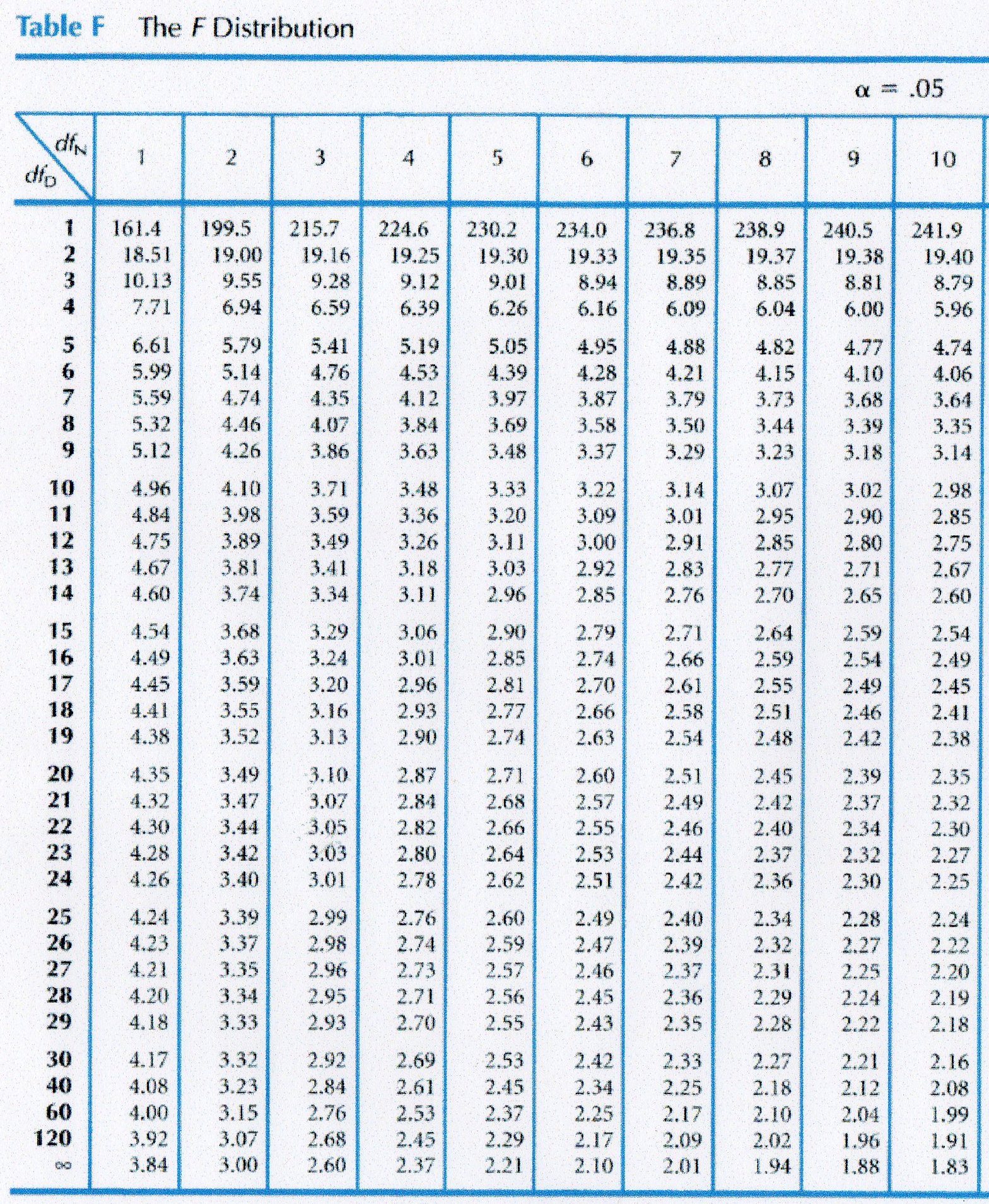
Just as with the R Table and the T Table, we use the F Table to find the critical value of the F ratio. All critical values are calculated for p < .05. The F Table uses the dfbg to find the proper column (shown as dfN to designate the Numerator of the F ratio) and uses the dfwg to find the proper row (shown as dfD to designate the Denominator of the F ratio). Where they meet is the critical value of F. If your calculated F value is larger than the critical F then the results are significant and we can reject the null hypothesis (p < .05). If your calculated F value is smaller than the critical F then the results are not significant and we fail to reject the null hypothesis.
For the data above our degrees of freedom for the between and within groups are 2 and 21 respectively. Therefore we can go to the F Table and go to column 2 and row 21 and determine that our critical F value is 3.47. Since our calculated F value was 4.976 we can say with confidence that our results are significant (at p < .05) and we can reject the null hypothesis.
Additional Links about the Concept that might help: